Imagine an Expert Advisor that does far more than execute static rules. Instead of following one fixed script forever, it studies market behavior, updates its own expectations, adapts to volatility shifts, and improves decision-making as new data arrives. This article explores a modern self-improving trading EA designed for changing markets.
The foundation of this approach comes from combining three powerful disciplines: the probability logic of Markov state transitions, the pattern-recognition ability of neural networks, and the protective mechanics of hedging-based trade management. When these elements are engineered together correctly, the result is not just another robot. It becomes an adaptive framework built to handle uncertainty.
Our internal development tests at 4xPip have shown why this concept matters. Strategies built on adaptive state recognition can achieve strong annualized performance while keeping drawdowns controlled, especially when paired with disciplined money management. More importantly, these systems can function in both slow ranging conditions and fast directional moves, two environments where many ordinary EAs fail.
Core Logic Behind the Model
Markov State Systems: Why the Present Can Contain the Past:
A common trading question is simple: how much historical data is truly needed to estimate what may happen next? Markov models offer a surprisingly elegant answer. If the current market state is defined correctly, then the present condition already contains the most relevant information needed for the next-step probability estimate.
A Markov process assumes that the next state depends mainly on the current state rather than the full sequence of prior events.
At first glance, this may seem to conflict with traditional technical analysis, where traders believe chart history repeats itself. But the key lies in how “state” is defined. If state only means price, the model is weak. If state means a complete market snapshot, it becomes much more powerful.
In our architecture, the current state can include trend direction, ATR-normalized movement, volatility pressure, relative price position, and behavior near recent highs or lows. That means prior market information is compressed into a usable present-state description.
The transition matrix then becomes a probability map. Each cell represents the chance of moving from one market condition to another. For algorithmic traders, this is extremely valuable because it converts raw price noise into measurable probabilities.
Neural Processing Layer: Interpreting Transition Patterns:
Once the state-transition matrix is built, we feed that data into a multilayer perceptron (MLP). This neural network acts as an interpreter. Instead of manually coding every market rule, the model learns relationships hidden inside transition probabilities.
Our standard architecture uses nine inputs from a 3×3 matrix, a hidden layer with forty neurons using ReLU activation, and two outputs representing bullish and bearish probabilities. This gives the system enough flexibility to capture nonlinear market behavior without becoming unnecessarily heavy.
The hidden layer is where the value emerges. Simple statistics may show state persistence or reversal frequency, but a neural network can detect combinations of conditions that humans often miss. It can recognize when a trending state followed by shrinking volatility tends to reverse, or when sideways compression often leads to expansion.
At 4xPip, our MQL developers regularly optimize these structures during testing on MT4 and MT5 environments. We focus heavily on performance stability rather than just curve-fitted profits, because real traders need robust execution across brokers and asset classes.
Turning Theory into a Functional EA
Identifying Current Market Conditions:
Every adaptive EA must first classify what type of market exists right now. Is price trending upward, declining, or moving sideways? We use ATR as a normalization tool so the logic adjusts naturally to different volatility conditions.
enum MARKET_STATE
{
  STATE_RANGE = 0,
  STATE_BULL  = 1,
  STATE_BEAR  = 2
};
int atrHandle;
MARKET_STATE GetMarketState(int shift)
{
  double close[];
  double atr[];
  ArraySetAsSeries(close,true);
  ArraySetAsSeries(atr,true);
  if(CopyClose(_Symbol, PERIOD_D1, shift, 2, close) < 2)
     return STATE_RANGE;
  if(CopyBuffer(atrHandle,0,shift,1,atr) < 1)
     return STATE_RANGE;
  double move = close[0] - close[1];
  double vol  = atr[0];
  if(move > 0.5 * vol)
     return STATE_BULL;
  if(move < -0.5 * vol)
     return STATE_BEAR;
  return STATE_RANGE;
}
This logic compares daily price movement against ATR rather than fixed pip values. That matters because a 50-point move may be huge in one market and insignificant in another. By scaling movement against volatility, the EA remains useful on Forex pairs, metals, crypto, and indices.
For traders, this means fewer manual adjustments. Our team at 4xPip builds systems specifically to save users from spending weeks recalibrating settings for each symbol.
The ATR handle is initialized during startup and released properly when the EA is removed.
int OnInit()
{
  atrHandle = iATR(_Symbol, PERIOD_D1, 14);
  if(atrHandle == INVALID_HANDLE)
     return INIT_FAILED;
  return INIT_SUCCEEDED;
}
void OnDeinit(const int reason)
{
  IndicatorRelease(atrHandle);
}
This ensures efficient memory use and stable platform operation. Clean initialization is especially important when traders run multiple charts or portfolios simultaneously.
Building the Probability Transition Matrix:
Once states are known, the EA studies how markets move between them. It records how often range becomes bullish, bullish remains bullish, bearish turns range, and so on.
double matrix[3][3];
int counts[3];
int flow[3][3];
void UpdateMatrix(int bars)
{
  ArrayInitialize(matrix,0);
  ArrayInitialize(counts,0);
  ArrayInitialize(flow,0);
  MARKET_STATE prev = GetMarketState(bars-1);
  for(int i=bars-2; i>=0; i--)
  {
    MARKET_STATE cur = GetMarketState(i);
     counts[prev]++;
     flow[prev][cur]++;
     prev = cur;
  }
  for(int r=0; r<3; r++)
  {
     for(int c=0; c<3; c++)
     {
        if(counts[r] > 0)
           matrix[r][c] = (double)flow[r][c] / counts[r];
        else
           matrix[r][c] = 1.0/3.0;
     }
  }
}
This routine converts historical sequences into probabilities. If bullish conditions often continue, the bullish-to-bullish cell becomes large. If ranges frequently break lower, the range-to-bearish probability rises.
Equal fallback probabilities are used when data is missing. That prevents distorted behavior when the sample window has not yet seen a specific state.
A sample EURUSD matrix might show high diagonal values, meaning states tend to persist. This often matches reality, where markets can remain trending or consolidating longer than traders expect.
Training the Neural Model:
The next layer is machine learning. We generate examples where the matrix values become inputs and future price direction becomes the target.
const int INPUTS  = 9;
const int OUTPUTS = 2;
CMLPBase mlp;
datetime lastTrain;
bool TrainModel()
{
  double close[];
  ArraySetAsSeries(close,true);
  int bars = CopyClose(_Symbol, PERIOD_CURRENT, 0, 5000, close);
  if(bars < 3000)
     return false;
  CMatrixDouble xy;
  xy.Resize(600, INPUTS + OUTPUTS);
  for(int i=0; i<600; i++)
  {
     UpdateMatrix(100);
     int k=0;
     for(int r=0; r<3; r++)
        for(int c=0; c<3; c++)
           xy.Set(i,k++,matrix[r][c]);
     double future = close[i] - close[i+24];
     xy.Set(i,INPUTS+0, future > 0 ? 1.0 : 0.0);
     xy.Set(i,INPUTS+1, future < 0 ? 1.0 : 0.0);
  }
  if(mlp.GetNeuronCount()==0)
  {
     int layers[] = {INPUTS,40,OUTPUTS};
     mlp.Create(layers,3);
  }
  int info=0;
  CMLPReportShell report;
  CAlglib::MLPTrainLBFGS(
     mlp,xy,600,0.001,5,0.01,100,info,report
  );
  lastTrain = TimeCurrent();
  return info >= 0;
}
This process teaches the model to associate certain probability structures with likely future movement. L-BFGS optimization is efficient and commonly used for numerical training tasks.
We also retrain regularly so the EA can adjust when market behavior changes. This is one of the most important benefits of self-learning systems: they are not trapped in old conditions.
At 4xPip, our programmers heavily emphasize backtesting and walk-forward optimization before release. We validate products across MT4, MT5, Forex brokers, stock brokers, crypto feeds, metals, commodities, and indices whenever possible.
Trade Decision Engine and Capital Control:
Once trained, the EA uses the neural output to decide whether to open buy or sell positions.
double lotSize      = 0.01;
int    maxTrades    = 5;
double gapPoints    = 50;
double tpPoints     = 100;
void OnTick()
{
  double in[9], out[2];
  UpdateMatrix(100);
  int x=0;
  for(int r=0; r<3; r++)
     for(int c=0; c<3; c++)
        in[x++] = matrix[r][c];
  CAlglib::MLPProcess(mlp,in,out);
  double buyProb  = out[0];
  double sellProb = out[1];
  if(buyProb > 0.55)
    trade.Buy(lotSize,_Symbol);
  if(sellProb > 0.55)
     trade.Sell(lotSize,_Symbol);
}
The thresholds prevent random entries. Only when the model shows sufficient confidence does the system act.
One powerful feature is the ability to hold both long and short positions when market conditions justify it. During highly volatile periods, both upside and downside probabilities may be elevated. In that case, hedged exposure can reduce directional risk.
Profitable positions may be closed quickly while opposing trades are managed carefully. This creates a structure where strong moves can be harvested while reversals remain tradable later.
Spacing logic between entries is also important. Without it, many EAs stack trades too close together and increase drawdown unnecessarily. Proper distance control creates smoother exposure.
Validation and Performance Review
After development, the next stage is real testing. We studied this model over historical data from 2017 through 2025 across major currency pairs and other liquid assets.
On EURUSD, optimized configurations showed strong returns with controlled drawdown. Metrics such as Sharpe ratio, profit factor, and recovery factor were competitive compared with many retail systems. More importantly, results were not dependent on one market phase only.
That is where adaptive models stand out. During volatile months, many static robots fail because their logic was tuned for quiet periods. A retrained neural-state system can adjust more quickly.
During strong USD moves in 2024, for example, directional pressure changed rapidly. Systems with rigid filters often struggled. Adaptive probability models had a better chance to respond because their transition behavior changed with new data.
This type of robustness is why our 4xPip development process focuses on practical survivability rather than marketing-only backtests.
Future Enhancements and Expansion Paths
Richer State Classification:
The three-state model is useful, but more detail can improve precision. Instead of bullish, bearish, and range only, markets can be divided into weak, moderate, and strong trend levels.
enum ADV_STATE
{
  STRONG_BEAR = 0,
  MID_BEAR    = 1,
  LIGHT_BEAR  = 2,
  RANGE       = 3,
  LIGHT_BULL  = 4,
  MID_BULL    = 5,
  STRONG_BULL = 6
};
This allows the matrix to capture not just direction, but intensity. A mild uptrend behaves differently from an explosive breakout.
Broader Technical Inputs:
ATR alone is valuable, but additional inputs can deepen market awareness. RSI can detect momentum exhaustion, MACD can highlight trend acceleration, and volume-based tools can confirm participation.
Combining multiple indicators gives the neural model a richer context. Instead of seeing only movement size, it can also see momentum quality and participation strength.
Smart Position Sizing:
Another major upgrade is dynamic lot allocation. When model confidence is high and risk conditions are favorable, exposure can increase modestly. When signals conflict, lot size can decrease.
This creates a more professional risk framework. Strong opportunities receive more capital, while uncertain periods preserve equity.
Multi-Timeframe Intelligence:
A further step is combining several chart horizons at once. Monthly and weekly trends can guide broader bias, while H1 or M15 charts provide tactical entries.
This creates alignment between macro direction and short-term timing. Traders often manually do this already; an advanced EA can automate it consistently.
Conclusion
This self-learning EA concept is more than a combination of separate tools. It merges statistical probability, machine learning, and practical trade management into one coherent framework.
By using Markov transitions to understand market behavior, neural networks to interpret probabilities, and hedging logic to manage uncertainty, the system becomes capable of operating in many different environments.
It is not a magic machine. Like any serious trading technology, it requires testing, parameter discipline, and sensible expectations. But when built correctly, it can become a valuable decision engine for both new and experienced traders.
At 4xPip, our goal is simple: help traders skip months of coding, trial-and-error testing, and platform frustration so they can move faster toward execution. Our MQL developers and quantitative programmers continue building advanced tools for MT4 and MT5 users who want smarter automation.
The future of algorithmic trading belongs to systems that learn, adapt, and improve. This model is one clear step in that direction.